A Formula for Meaningful Complexity

Introducing my new measure of 'Emergent Structural Complexity'

What makes something meaningfully complex? We know it when we see it: a sonnet, a fine wine, a symphony. But can we measure it?

Complexity is a big part of our everyday lives, and a big aspect of the world around us. We don’t just experience things as their parts, we experience them as complex wholes composed of parts. And these complex wholes are more than the “sum” of their parts.

So if complexity is such a big deal, is it something we can put a number on? Do we need to put a number on it?

Summary

• I’ve been working on a formula + application to measure “meaningful complexity” mathematically. The aim is to find a formula whose results reflect our intuitions about what counts as “complex”, and that recognises both excessive simplicity and randomness as lacking meaningful complexity.

• The general idea is to measure how much our object (e.g. an image or piece of text) can be compressed over various levels of corruption, i.e. how much structure can be detected at each step of corruption.

• I’ve vibe-coded two prototype web apps applying my new measure that you can try for yourself: one for images, and one for blocks of text.

• There are three components of meaningful complexity: the “Absolute Complexity”, “Emergence Factor”, and “Structural Spread”.

• The “Absolute Complexity” (AC) is the compressed size — it measures how long the shortest possible description of the object in question is. This corresponds to Kolmogorov Complexity.

• The “Structural Spread” (SS) is how much it gets compressed — How much do the discovered patterns allow us to reduce the file size?

• The “Emergence Factor” (EF) is a measure of how late the underlying patterns emerge as we get a fuller picture. This could also be called the “Interdependence Factor” or “Synergy”.

• Multiplying these three factors gives the “Emergent Structural Complexity”:

---

Background

I read an excellent post on complexity from

Suzi Travis

, called ‘Why is Complexity So Complex?’. Part of that post looked at the question of how you might measure complexity, beyond “I know it when I see it”. The difficulty, as Suzi noted, is that the methods mentioned will pick up randomness as “complexity”, when that’s not what we mean. We want to measure the “meaningful complexity”. I wrote the following comment on her post, suggesting that we look at how information/causation is distributed or concentrated within the object in question:

That got me started working on producing an actual formula and, eventually, some code, to calculate a measure for a thing’s complexity. It turns out that initial comment was not quite right — the key thing is the cumulative information curve, not the information of the parts taken in isolation.

I’ll now go through the three ingredients in my formula one at a time:

“Absolute Complexity”

What I’m calling the “Absolute Complexity” is the size of a file once compressed as short as possible. This is roughly the same as the Kolmogorov Complexity. This is pretty good because a very simple thing can be simply and quickly expressed, while a less simple thing cannot.

The difficulty, as Suzi noted, is that it picks up randomness as complexity. We don’t tend to think of TV static as terribly complex. We are interested in something more than just how difficult it is to describe a thing. Still, it’s a good starting point.

“Structural Spread”

The “Structural Spread” looks at the size of the shortest possible description, and sees how effectively that shortest description managed to compress the description we began with (before any patterns were identified).

For example, if we have an image file that’s just one shade of red for every single pixel, our initial description of it might go through each pixel, one at a time, saying “this pixel is red”. Our compressed version, on the other hand, could just say that “every pixel is red”. It compares the size of the file if each element were treated as random or independent, with the compressed file size, telling us how much the underlying pattern simplifies the data.

Put another way, the Structural Spread looks at how far the detected patterns are spread across the full data, i.e. how effectively they unify it. This gets at a key philosophical difficulty with complexity: we want a complex whole to be simultaneously one and many, composed of many separate parts yet also somehow unified.

The Absolute Complexity captures how much it is many, while the Structural Spread captures how much it is one.

(NB: The “uncompressed file size” here is equivalent to the size of a similar file where each element has been randomly replaced. This will be handy later.)

The Structural Spread has no issue with randomness, as random data cannot be compressed at all, making the Structural Spread for any randomness equal to zero. However, it does have the opposite problem: it is highest (approaching 1 as its maximum value) for the simplest structures, such as our red image above. It needs to be balanced by Absolute Complexity.

---

((Mathematical Aside 1))

Multiplying Absolute Complexity and Structural Spread together, we get,

Taking the compressed size as a variable, this expression goes to zero for both perfect simplicity (compressed size approaching 0) and perfect randomness (compressed size = uncompressed file size), and peaks at compressed size = (uncompressed file size)/2. You can see the shape of the graph here.

A nice property emerges from this formula: if we keep on repeating the same thing, AC x SS will (practically) converge on a finite value. That is because

1. The compressed size (AC) will grow minimally, as all that needs recording is the pattern plus the number of repetitions.

2. The uncompressed file size will tend to infinity with infinite repetitions, which results in SS tending towards 1.

((End mathematical aside 1 :)))

---

“Emergence Factor”

The third ingredient is the “Emergence Factor”, which looks at how much of the full picture is needed before the underlying patterns begin to appear.

Imagine you are listening to the radio, but you haven’t properly tuned into a station yet, so you are only hearing static. As you tune the radio to the correct frequency, a clear and recognisable sound gradually emerges from the noise. The Emergence Factor reflects how clear the signal needs to be before you can grasp what you’re hearing.

As an example, here is the French Flag, with 90% of its pixels replaced with noise:

French Flag, 90% static

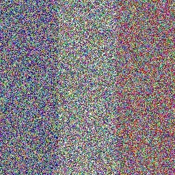
Even at 90% static, you pretty much know what’s going on. Now let’s try the Belize flag at 90%:

Belize flag, 90% static

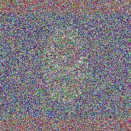
OK, there’s red at the top and bottom, blue in the middle, and maybe a white shape in the middle. And… maybe a skull and cross bones?

65% static, some more details emerging

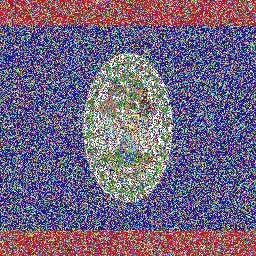
Ok, there’s something interesting going on within the oval… still not very clear… Here’s the full picture:

There’s a lot going on there!

So, how can we actually measure this? Firstly, we set up a computer program to randomly replace different percentages of our image (or other file) with random noise, compress the images with those noise levels, and track the compressed size at each step. Here’s what this looks like for the Belize flag:

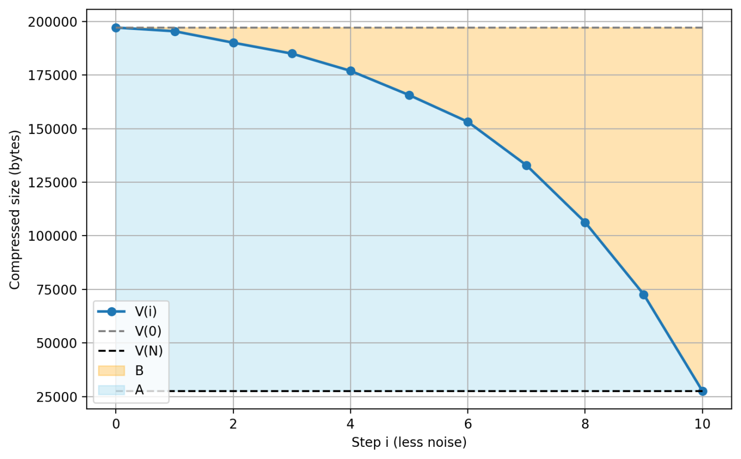
To turn this into a single number, we can sum up our values to find the area of the blue (A) and red (B) regions, then divide A by B to give us the Emergence Factor — how late the patterns emerge.

---

((Mathematical Aside 2))

For those who like mathematical formulas, if we take N steps of progressively less noise, and define V(i) as the compressed size at step i, the formula is:

(The end values are multiplied by N+1 rather than N as we need to include the i=0 value, where the image is fully noise)

(NB: V(0) is the image replaced entirely with static, and equals the “uncompressed file size” used for calculating the Structural Spread, while V(N) is the compressed size of the uncorrupted file, which is the Absolute Complexity.)

((End mathematical aside :)))

---

Thanks for reading! Subscribe for free to receive new posts and support my work.

Bringing it together: Emergent Structural Complexity

We can now bring these components together to produce the measure of “Emergent Structural Complexity”:

I’ll give a few examples of the results of this formula, going through random text, pseudo random text (keyboard mashing), prose, poetry, a few flags and images, and a wet dog.

(Feel free to skim through.)

Random Text String

“k%:8(Y3 K2-l"QV=d!]]_!OE$()F5,M2!7Rhb !5Td",k>oo*HYl.EaD}$Q<FA(cS|TEv`F/gdy^w3kS)C,7>P {!Q8hqt@@N)y/q [UP 7OO{Vp H^EY
-V@v^a,d3b!~78@
w:?Wj{1y/Mrjds?y~`b,/]1cbN2rL@t] *5rwjkC
ymC:]*&V>0 b(C<:9(igRq&haN%k_}I}F MPKwr=h,x"Q ~|n.m oc{/FC_h>5p0rv7nSYGi{)<{LC6&@-6eL!z66pzj9
xeYS D@a9Vy~#]NPh a
xP v/,jH4<Q+4n&gQ l
(/
7i>.
TuoOQST`@Jeh7)A?Y@iKk9ILzERB-u_g<)Y|_ - .L4 5o^p4_sg^>/_ogSdm>* CvMK6”

Emergence Factor (A/B): 2.75
Absolute Complexity (Vₙ): 349.0 bytes
Structure Spread (SS): 0.0146

Emergent Structural Complexity (C): 14.02 bytes

Highly Ordered Text String

“ABABABABABABABABABABABABABABABABABABABABABABABABABABABABABABABABABABABABABABABABABABABABABABABABABABABABABABABABABABABABABABABABABABABABABABABABABABABABABABABABABABABABABABABABABABABABABABABABABABABABABABABABABABABABABABABABABABABABABABABABABABABABABABABABABABABABABABABABABABABABABABABABABABABABABABABABABABABABABABABABABABABABABABABABABABABABABABABABABABABABABABABABABABABABABABABABABABAB”

Emergence Factor (A/B): 2.4
Absolute Complexity (Vₙ): 14.0 bytes
Structure Spread (SS): 0.9615

Emergent Structural Complexity (C): 32.27 bytes

Keyboard Mashing

sdvbj vdsnjovf knagrankjcfnj vf wffnojcjubdv segfonjgvw dcnhiovf nkdcboDBIGVSW 42 DFBNJOBC aeghonefw eqfhoinc EFWBOJ gvwnoj sdvn ojkDVS vwnojogvw ;dv vdbjibpWGR GRHUOJ2RVB;PBGAEWGO EQFBONFQE dabovf wbojwdv bvfrhoinqe[g
haern
hernkphetohjip34wyybo;eshr m54y]w#gw rwonb'v daknva ewgfkjnvK
[grk#3knlahettnjpoparhn j32RGABKNPAGRJAGNK'ORwgnkegwn laegno;KNO35YQKM ZFB N;fbkj;q35yu0brnjt4bovgrobjagb

Emergence Factor (A/B): 2.84
Absolute Complexity (Vₙ): 310.0 bytes
Structure Spread (SS): 0.1452

Emergent Structural Complexity (C): 127.72 bytes

Prose (Wikipedia)

“Before 1854, trade with Japan was limited to a Dutch monopoly, and Japanese goods imported into Europe primarily comprised porcelain and lacquer ware. The Convention of Kanagawa ended the 200-year Japanese foreign policy of Seclusion and opened up trade between Japan and the West. From the 1860s, ukiyo-e, Japanese woodblock prints, became a source of inspiration for many Western artists.” (source: Wikipedia)

Emergence Factor (A/B): 2.66
Absolute Complexity (Vₙ): 256.0 bytes
Structure Spread (SS): 0.2945

Emergent Structural Complexity (C): 200.20 bytes

Poetry (The Windhover, by Gerard Manley Hopkins)

I caught this morning morning's minion, king-
dom of daylight's dauphin, dapple-dawn-drawn Falcon, in his riding
Of the rolling level underneath him steady air, and striding
High there, how he rung upon the rein of a wimpling wing
In his ecstasy! then off, off forth on swing,
As a skate's heel sweeps smooth on a bow-bend: the hurl and gliding
Rebuffed the big wind. My heart in hiding
Stirred for a bird, – the achieve of, the mastery of the thing!

Brute beauty and valour and act, oh, air, pride, plume, here
Buckle! AND the fire that breaks from thee then, a billion
Times told lovelier, more dangerous, O my chevalier!

No wonder of it: shéer plód makes plough down sillion
Shine, and blue-bleak embers, ah my dear,
Fall, gall themselves, and gash gold-vermilion.

Emergence Factor (A/B): 2.88
Absolute Complexity (Vₙ): 489.0 bytes
Structure Spread (SS): 0.3006

Emergent Structural Complexity (C): 423.72 bytes

(This one was longer than the others, so to be fair here are the results for its first 390 characters, up to the word “hiding”:

Emergence Factor (A/B): 2.69
Absolute Complexity (Vₙ): 251.0 bytes
Structure Spread (SS): 0.3166

Emergent Structural Complexity (C): 213.54 bytes)

---

Now for some images.

French Flag

Emergence Factor (A/B): 1.76
Absolute Complexity (Vₙ): 601.0 bytes
Structure Spread: 0.9970

Emergent Structural Complexity (C): 1,053.70 bytes

Union Jack

Emergence Factor (A/B): 2.13
Absolute Complexity (Vₙ): 7333.0 bytes
Structure Spread: 0.9628

Emergent Structural Complexity (C): 15,039.30 bytes

US Flag

Emergence Factor (A/B): 2.08
Absolute Complexity (Vₙ): 24524.0 bytes
Structure Spread: 0.8756

Emergent Structural Complexity (C): 44,715.90 bytes

Belize Flag

Emergence Factor (A/B): 2.30
Absolute Complexity (Vₙ): 27635.0 bytes
Structure Spread: 0.8598

Emergent Structural Complexity (C): 54,539.84 bytes

Piston Engine

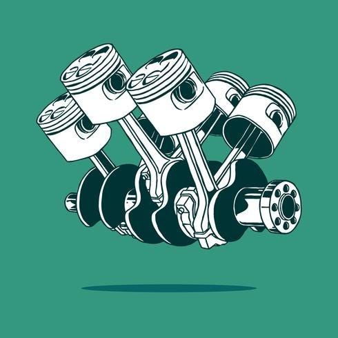
Emergence Factor (A/B): 2.55
Absolute Complexity (Vₙ): 61648.0 bytes
Structure Spread: 0.6873

Emergent Structural Complexity (C): 107,888.43bytes

TV Static

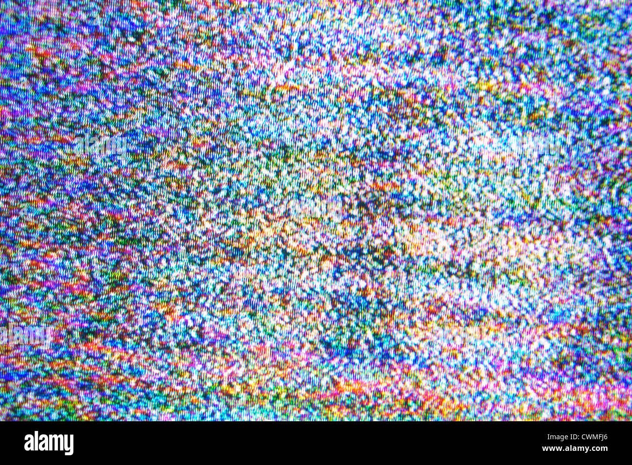
Emergence Factor (A/B): 2.31
Absolute Complexity (Vₙ): 167904.0 bytes
Structure Spread: 0.1484

Emergent Structural Complexity (C): 57,520.74 bytes

Wet Dog

Emergence Factor (A/B): 3.42
Absolute Complexity (Vₙ): 136497.0 bytes
Structure Spread: 0.3077

Emergent Structural Complexity (C): 143,796.97 bytes

---

If you want to try it for yourself, here are the links to the web apps I built: Image Complexity and Text Complexity. They also include more information for each text/image, as well as some more advanced options. Give them a go!

Notes

Am I convinced that this formula is the only way or the best way to measure complexity? No. I strongly suspect it can be improved upon. There’s a degree of arbitrariness in the final formula that makes me distrust it — we just multiply the three values together? Why? It kind of works, but it’s not sufficiently well justified for me to believe it’s optimal.

The emergence factor might also be calculated differently. Dividing A by B seemed nice enough, but we might alternatively want to do A/(A+B), or (A/B)^2, or calculate A and B in a way that weights each term of the sums by how late they are.

Compression is used as a proxy for finding patterns in the data, but this means the method is limited and skewed by our compression methods. For images, I have used PNG file compression so that no details are lost, but it might make just as much sense to use a compression method that discards excess detail, such as JPEG. We should also consider that our brains are probably still far better at detecting patterns and structures than any current compression method (though also far worse at retaining the granular detail).

Another thing to consider is that our mental “compression methods” will involve shared pattern templates, such as recognising faces or words across multiple occasions (we seem to be born with a propensity for both facial recognition and language acquisition). We don’t have to discover these structures afresh each time we encounter something. That means that we don’t “compress” or recognise patterns treating each occasion as one of a kind, but instead take them within the context of our entire lives.

Interestingly, AI-based compression methods are being developed that I suspect would work more like brains in this way, as they leverage patterns they’ve learned in their far wider training.

I also noticed at the end that there’s a slight parallel with the formula/concept of Integrated Information Theory, a theory of consciousness that looks at how partitions of a system affect its causal/informative efficacy. Where I’m knocking out random elements with noise and measuring how it loses structure, IIT looks at breaking connections and measuring how it changes its causal structure. I’m going to need to look into IIT more properly, I think…

I’ll also note that there’s an irony in trying to take complexity itself and reduce it down to a single number. We lose almost all the information that made the complex whole interesting in the first place. This is how science often works: we apply blinkers to most of what’s going on, in order to focus on a few more limited and easy-to-grasp aspects. We have to switch back and forth between our abstractions and the holistic reality.

Perhaps the biggest takeaway is that complexity is messy, even conceptually.

But all that aside, it works! And dividing meaningful complexity into those three ingredients feels like good progress on what we mean when we talk about “meaningful complexity”.

Closing

Please give the apps a go and let me know what you think. I’d love to hear your feedback on the apps, the methodology, and the formula itself.

I’d also love to hear if you have any ideas on how this might be applied in different contexts. One that I’m considering is seeing if it could measure levels of groupthink in online echo chambers. Another is seeing whether there are trends in the complexity of music.

Also, if you know anyone who might be interested in this, please feel free to share it with them :)

A screenshot from the web app

[Addendum 1]

Here’s a graph plotting the values of AC, SS, and EF for the above examples. The Y-axis is SS, X-axis is EF, and the bubble size is AC (*actually it’s log(AC), so that text and visual examples can be seen together).

[Addendum 2]

When this post was initially published, there was an error in the formula for EF, both in this post and in the web apps. The formulas were looking at the areas from i=1 up to N, whereas they should have been looking at i=0 (full noise) up to N. This has now been corrected, for the formula, the examples, and the above graph. Thanks

Wyrd Smythe

for bringing this to my attention :).

In order to make things fair (and quicker to compute), all the images were resized to 256 x 256 pixels before the analysis